withPoints - Category
When points are added to the graph.
Warning
Proposed functions for next mayor release.
They are not officially in the current release.
They will likely officially be part of the next mayor release:
The functions make use of ANY-INTEGER and ANY-NUMERICAL
Name might not change. (But still can)
Signature might not change. (But still can)
Functionality might not change. (But still can)
pgTap tests have being done. But might need more.
Documentation might need refinement.
withPoints - Family of functions - Functions based on Dijkstra algorithm.
From the TRSP - Family of functions:
pgr_trsp_withPoints - Proposed - Vertex/Point routing with restrictions.
pgr_trspVia_withPoints - Proposed - Via Vertex/point routing with restrictions.
Introduction
The with points category modifies the graph on the fly by adding points on edges as required by the Points SQL query.
The functions within this category give the ability to process between arbitrary points located outside the original graph.
This category of functions was thought for routing vehicles, but might as well work for some other application not involving vehicles.
When given a point identifier pid that its being mapped to an edge with an
identifier edge_id, with a fraction from the source to the target along the
edge fraction and some additional information about which side of the edge
the point is on side, then processing from arbitrary points can be done on
fixed networks.
All this functions consider as many traits from the “real world” as possible:
Kind of graph:
directed graph
undirected graph
Arriving at the point:
Compulsory arrival on the side of the segment where the point is located.
On either side of the segment.
Countries with:
Right side driving
Left side driving
Some points are:
Permanent: for example the set of points of clients stored in a table in the data base.
The graph has been modified to permanently have those points as vertices.
There is a table on the database that describes the points
Temporal: for example points given through a web application
Use pgr_findCloseEdges in the Points SQL.
The numbering of the points are handled with negative sign.
This sign change is to avoid confusion when there is a vertex with the same identifier as the point identifier.
Original point identifiers are to be positive.
Transformation to negative is done internally.
Interpretation of the sign on the node information of the output
positive sign is a vertex of the original graph
negative sign is a point of the Points SQL
Parameters
Column |
Type |
Description |
|---|---|---|
|
Edges SQL as described below |
|
|
Points SQL as described below |
|
|
Combinations SQL as described below |
|
start vid |
|
Identifier of the starting vertex of the path. Negative value is for point’s identifier. |
start vids |
|
Array of identifiers of starting vertices. Negative values are for point’s identifiers. |
end vid |
|
Identifier of the ending vertex of the path. Negative value is for point’s identifier. |
end vids |
|
Array of identifiers of ending vertices. Negative values are for point’s identifiers. |
Optional parameters
Parameter |
Type |
Default |
Description |
|---|---|---|---|
|
|
|
Value in [
|
|
|
|
|
Inner Queries
Edges SQL
Column |
Type |
Default |
Description |
|---|---|---|---|
|
ANY-INTEGER |
Identifier of the edge. |
|
|
ANY-INTEGER |
Identifier of the first end point vertex of the edge. |
|
|
ANY-INTEGER |
Identifier of the second end point vertex of the edge. |
|
|
ANY-NUMERICAL |
Weight of the edge ( |
|
|
ANY-NUMERICAL |
-1 |
Weight of the edge (
|
Where:
- ANY-INTEGER:
SMALLINT,INTEGER,BIGINT- ANY-NUMERICAL:
SMALLINT,INTEGER,BIGINT,REAL,FLOAT
Points SQL
Parameter |
Type |
Default |
Description |
|---|---|---|---|
|
ANY-INTEGER |
value |
Identifier of the point.
|
|
ANY-INTEGER |
Identifier of the “closest” edge to the point. |
|
|
ANY-NUMERICAL |
Value in <0,1> that indicates the relative postition from the first end point of the edge. |
|
|
|
|
Value in [
|
Where:
- ANY-INTEGER:
SMALLINT,INTEGER,BIGINT- ANY-NUMERICAL:
SMALLINT,INTEGER,BIGINT,REAL,FLOAT
Combinations SQL
Parameter |
Type |
Description |
|---|---|---|
|
ANY-INTEGER |
Identifier of the departure vertex. |
|
ANY-INTEGER |
Identifier of the arrival vertex. |
Where:
- ANY-INTEGER:
SMALLINT,INTEGER,BIGINT
Advanced documentation
About points
For this section the following city (see Sample Data) some interesing points such as restaurant, supermarket, post office, etc. will be used as example.
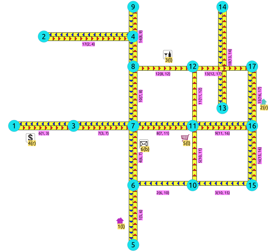
The graph is directed
Red arrows show the
(source, target)of the edge on the edge tableBlue arrows show the
(target, source)of the edge on the edge tableEach point location shows where it is located with relation of the edge
(source, target)On the right for points 2 and 4.
On the left for points 1, 3 and 5.
On both sides for point 6.
The representation on the data base follows the Points SQL description, and for this example:
SELECT pid, edge_id, fraction, side FROM pointsOfInterest;
 pid | edge_id | fraction | side
-----+---------+----------+------
   1 |       1 |      0.4 | l
   2 |      15 |      0.4 | r
   3 |      12 |      0.6 | l
   4 |       6 |      0.3 | r
   5 |       5 |      0.8 | l
   6 |       4 |      0.7 | b
(6 rows)
Driving side
In the the folowwing images:
The squared vertices are the temporary vertices,
The temporary vertices are added according to the driving side,
visually showing the differences on how depending on the driving side the data is interpreted.
Right driving side
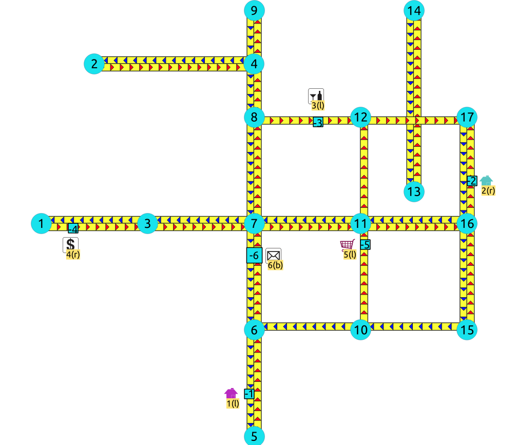
Point 1 located on edge
(6, 5)Point 2 located on edge
(16, 17)Point 3 located on edge
(8, 12)Point 4 located on edge
(1, 3)Point 5 located on edge
(10, 11)Point 6 located on edges
(6, 7)and(7, 6)
Left driving side
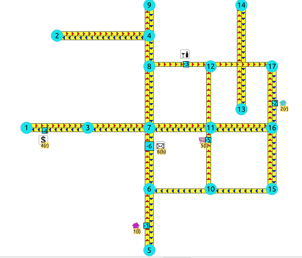
Point 1 located on edge
(5, 6)Point 2 located on edge
(17, 16)Point 3 located on edge
(8, 12)Point 4 located on edge
(3, 1)Point 5 located on edge
(10, 11)Point 6 located on edges
(6, 7)and(7, 6)
Driving side does not matter
Like having all points to be considered in both sides
bPrefered usage on undirected graphs
On the TRSP - Family of functions this option is not valid
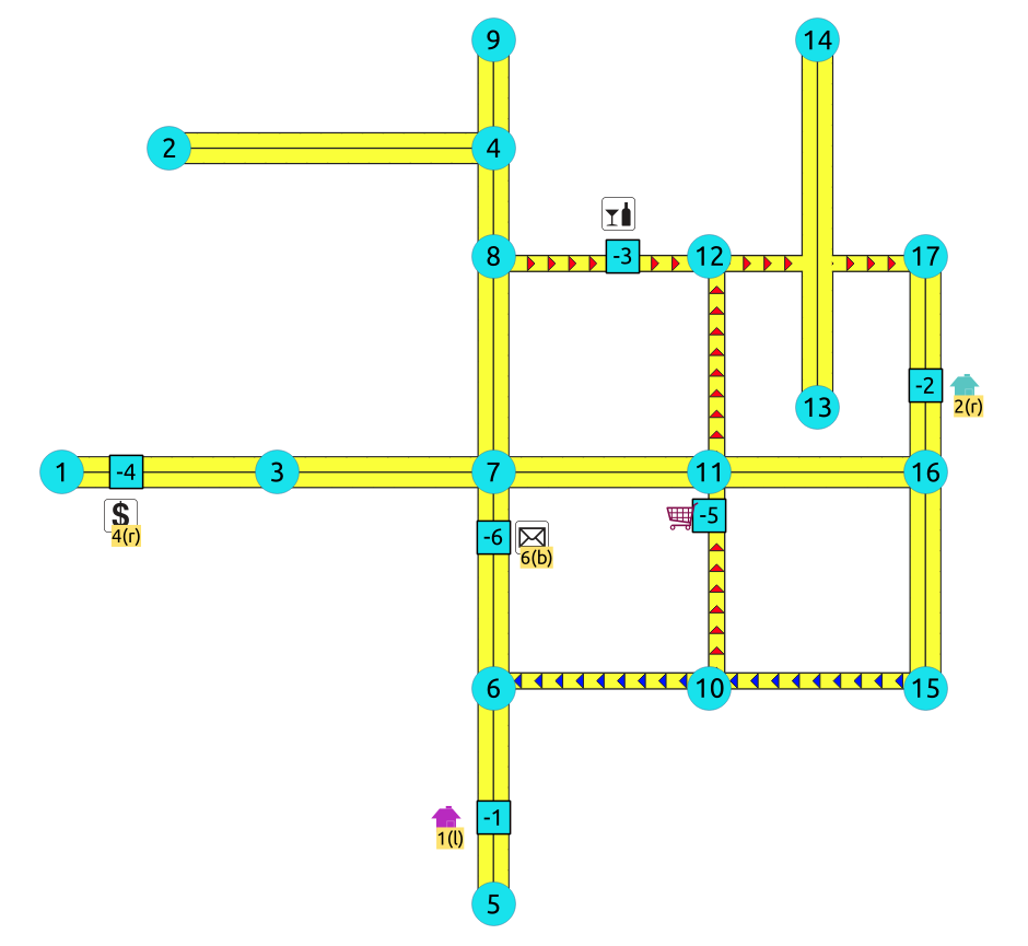
Point 1 located on edge
(5, 6)and(6, 5)Point 2 located on edge
(17, 16)``and ``16, 17Point 3 located on edge
(8, 12)Point 4 located on edge
(3, 1)and(1, 3)Point 5 located on edge
(10, 11)Point 6 located on edges
(6, 7)and(7, 6)
Creating temporary vertices
This section will demonstrate how a temporary vertex is created internally on the graph.
Problem
For edge:
SELECT id, source, target, cost, reverse_cost
FROM edges WHERE id = 15;
 id | source | target | cost | reverse_cost
----+--------+--------+------+--------------
 15 |     16 |     17 |    1 |            1
(1 row)
insert point:
SELECT pid, edge_id, fraction, side
FROM pointsOfInterest WHERE pid = 2;
 pid | edge_id | fraction | side
-----+---------+----------+------
   2 |      15 |      0.4 | r
(1 row)
On a right hand side driving network
Right driving side
Arrival to point
-2can be achived only via vertex 16.Does not affects edge
(17, 16), therefore the edge is kept.It only affects the edge
(16, 17), therefore the edge is removed.Create two new edges:
Edge
(16, -2)with cost0.4(original cost * fraction ==Edge
(-2, 17)with cost0.6(the remaing cost)
The total cost of the additional edges is equal to the original cost.
If more points are on the same edge, the process is repeated recursevly.
On a left hand side driving network
Left driving side
Arrival to point
-2can be achived only via vertex 17.Does not affects edge
(16, 17), therefore the edge is kept.It only affects the edge
(17, 16), therefore the edge is removed.Create two new edges:
Work with the original edge
(16, 17)as the fraction is a fraction of the original:Edge
(16, -2)with cost0.4(original cost * fraction ==Edge
(-2, 17)with cost0.6(the remaing cost)If more points are on the same edge, the process is repeated recursevly.
Flip the Edges and add them to the graph:
Edge
(17, -2)becomes(-2, 16)with cost0.4and is added to the graph.Edge
(-2, 16)becomes(17, -2)with cost0.6and is added to the graph.
The total cost of the additional edges is equal to the original cost.
When driving side does not matter
Arrival to point
-2can be achived via vertices 16 or 17.Affects the edges
(16, 17)and(17, 16), therefore the edges are removed.Create four new edges:
Work with the original edge
(16, 17)as the fraction is a fraction of the original:Edge
(16, -2)with cost0.4(original cost * fraction ==Edge
(-2, 17)with cost0.6(the remaing cost)If more points are on the same edge, the process is repeated recursevly.
Flip the Edges and add all the edges to the graph:
Edge
(16, -2)is added to the graph.Edge
(-2, 17)is added to the graph.Edge
(16, -2)becomes(-2, 16)with cost0.4and is added to the graph.Edge
(-2, 17)becomes(17, -2)with cost0.6and is added to the graph.
See Also
Indices and tables