pgr_contractionHierarchies - 实验性

pgr_contractionHierarchies — 根据收缩层级方法执行图收缩，并返回收缩后的顶点和生成的快捷边。

可用性

• Version 3.8.0

  • 新 实验性 函数

描述

收缩层次法是从顶点的初始顺序出发建立层次顺序的，在最短路径算法的标签固定处理过程中优先考虑某些顶点。此外，收缩层次算法还能在图中添加捷径边，帮助最短路径算法遵循所创建的层次图结构。

层次结构的原理是将属于长距离网络（例如公路网络中的高速公路）的顶点置于高优先级，而将属于短距离网络（例如公路网络中的主干道或次干路）的节点置于低优先级。

收缩层次结构算法的假设是，已经存在一个有价值的顶点顺序，用于初始化收缩过程。由于大多数情况下没有有价值的初始节点排序，因此我们使用顶点 ID 给出的顺序。然后，在这个首序的基础上进行收缩处理，得到最终的层次结构。

其基本原理是将顶点按其收缩吸引力的估计值排序，保留在优先队列中。实施案例中使用的度量称为 边差 ，相当于顶点收缩产生的捷径数量与收缩前图中附带边的数量之差 (#shortcuts - #incident edges).

最后，在使用类似 Dijkstra 的双向算法时，目的是减少图中已探索的部分。顶点顺序用于为定向搜索提供信息。搜索过程不会失去最优性。

为收缩寻找最佳顶点排序是一个难题。然而，根据 Geisberger 等人的研究 [2]，非常简单的局部启发式方法就能很好地解决这个问题。这种方法的原理是先验地估算 边差 的值，只有当新的度量值使位于队列顶端的节点保持在队列顶端时，才对其进行收缩。否则，它就会被重新插入队列，位于与新度量值相对应的正确位置。

这个过程是在只有边的成本为正值的图形上完成的。

需要注意的是，此函数不会删除任何顶点。最终图中保留了原有的所有顶点，但新增了一些对应于快捷边的边。为构建这些快捷边而收缩的顶点也会被保留，并按层级顺序排列。

至于其他收缩方法，它不会返回完整的收缩图，只会返回变化。它们有两种类型：

• 增加了带有负标识符的快捷边；

• 带有顺序的收缩节点。

Boost 图内部

签名

总结

pgr_contractionHierarchies 函数具有以下签名：

pgr_contractionHierarchies(Edges SQL, [options])

options: [directed, forbidden]

返回集合 (type, id, contracted_vertices, source, target, cost)

参数

参数	类型	描述
Edges SQL	TEXT	Edges SQL 如下所述。

可选参数

列	类型	默认	描述
directed	BOOLEAN	true	当 true 时，该图被视为有 有向 如果为 false ，则该图被视为 无向 。

收缩层级的可选参数

列	类型	默认	描述
forbidden	ARRAY[ ANY-INTEGER ]	Empty	禁止收缩的顶点标识符。
directed	BOOLEAN	$1$	如果图是有向的，则为 True，否则为 False。

内部查询

Edges SQL

列	类型	默认	描述
id	ANY-INTEGER		边的标识符。
source	ANY-INTEGER		边的第一个端点顶点的标识符。
target	ANY-INTEGER		边的第二个端点顶点的标识符。
cost	ANY-NUMERICAL		edge (source, target)的权重
reverse_cost	ANY-NUMERICAL	-1	边(target, source)的权重 当为负时：edge (target, source) 不存在，因此它不是图的一部分。

其中：

ANY-INTEGER:

SMALLINT, INTEGER, BIGINT

ANY-NUMERICAL:

SMALLINT, INTEGER, BIGINT, REAL, FLOAT

结果列

返回集合 (type, id, contracted_vertices, source, target, cost)

该函数返回多行（每个顶点一行，每创建一条快捷边一行）。行的列数为：

列	类型	描述
type	TEXT	id 的类型。 当该行表示一个顶点时，列为 v 。 列 id 为正值 当行是边时，则为 e 。 列 id 的值为负数
id	BIGINT	此列中的所有数字都是 DISTINCT 当 type = 'v' 时。 修改顶点的标识符。 当 type = 'e' 时。 从 -1 开始递减序列。 表示未包含在原始边集中的伪`id` 。
contracted_vertices	ARRAY[BIGINT]	收缩顶点标识符数组。
source	BIGINT	当 type = 'v': $-1$ 时 当 type = 'e' 时：当前边 (source, target) 的source顶点标识符。
target	BIGINT	当 type = 'v': $-1$ 时 当 type = 'e' 时：当前边 (source, target) 的target 顶点标识符。
cost	FLOAT	当 type = 'v': $-1$ 时 当 type = 'e' 时：当前边 (source, target) 的权重。
metric	BIGINT	当 type = 'v': $-1$ 时 当 type = 'e' 时：当前边 (source, target) 的权重。
vertex_order	BIGINT	当 type = 'v': $-1$ 时 当 type = 'e' 时：当前边 (source, target) 的权重。

示例

在无向图上

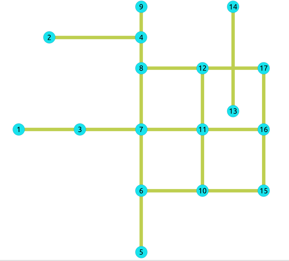
下面的查询显示了在无向图上进行收缩操作所涉及的原始数据。

SELECT id, source, target, cost FROM edges ORDER BY id;
 id | source | target | cost
----+--------+--------+------
  1 |      5 |      6 |    1
  2 |      6 |     10 |   -1
  3 |     10 |     15 |   -1
  4 |      6 |      7 |    1
  5 |     10 |     11 |    1
  6 |      1 |      3 |    1
  7 |      3 |      7 |    1
  8 |      7 |     11 |    1
  9 |     11 |     16 |    1
 10 |      7 |      8 |    1
 11 |     11 |     12 |    1
 12 |      8 |     12 |    1
 13 |     12 |     17 |    1
 14 |      8 |      9 |    1
 15 |     16 |     17 |    1
 16 |     15 |     16 |    1
 17 |      2 |      4 |    1
 18 |     13 |     14 |    1
(18 rows)

原始图：

示例:

在整个图形上建立收缩层次结构

SELECT * FROM pgr_contractionHierarchies(
  'SELECT id, source, target, cost FROM edges',
  directed => false);
 type | id | contracted_vertices | source | target | cost | metric | vertex_order
------+----+---------------------+--------+--------+------+--------+--------------
 v    |  1 | {}                  |     -1 |     -1 |   -1 |     -1 |            3
 v    |  2 | {}                  |     -1 |     -1 |   -1 |     -1 |           10
 v    |  3 | {}                  |     -1 |     -1 |   -1 |     -1 |            4
 v    |  4 | {}                  |     -1 |     -1 |   -1 |      0 |           15
 v    |  5 | {}                  |     -1 |     -1 |   -1 |     -1 |           14
 v    |  6 | {}                  |     -1 |     -1 |   -1 |     -1 |            6
 v    |  7 | {}                  |     -1 |     -1 |   -1 |     -1 |            5
 v    |  8 | {}                  |     -1 |     -1 |   -1 |     -1 |            9
 v    |  9 | {}                  |     -1 |     -1 |   -1 |     -2 |            2
 v    | 10 | {}                  |     -1 |     -1 |   -1 |     -1 |            7
 v    | 11 | {}                  |     -1 |     -1 |   -1 |     -1 |            8
 v    | 12 | {}                  |     -1 |     -1 |   -1 |     -2 |            1
 v    | 13 | {}                  |     -1 |     -1 |   -1 |     -1 |           11
 v    | 14 | {}                  |     -1 |     -1 |   -1 |      0 |           16
 v    | 15 | {}                  |     -1 |     -1 |   -1 |     -1 |           13
 v    | 16 | {}                  |     -1 |     -1 |   -1 |     -1 |           12
 v    | 17 | {}                  |     -1 |     -1 |   -1 |      0 |           17
 e    | -1 | {7}                 |     11 |      8 |    2 |     -1 |           -1
 e    | -2 | {7,8}               |     11 |      9 |    3 |     -1 |           -1
 e    | -3 | {8}                 |     12 |      9 |    2 |     -1 |           -1
 e    | -4 | {11}                |     12 |     16 |    2 |     -1 |           -1
(21 rows)

结果并不代表收缩后的图形。它们代表的是应用收缩算法后对图所做的改变，并根据 边差 度量对顶点进行排序，从而给出算法建立的顶点顺序。因此，结果中包含了所有顶点（当然禁止的顶点除外）。结果中只显示算法建立的捷径。

计算完收缩层次后，现在要给顶点排序，

是为了与一种特定的 Dijkstra 算法（在未来版本中实现）配合使用，从而加快搜索速度。

我们得到了上面的收缩图：

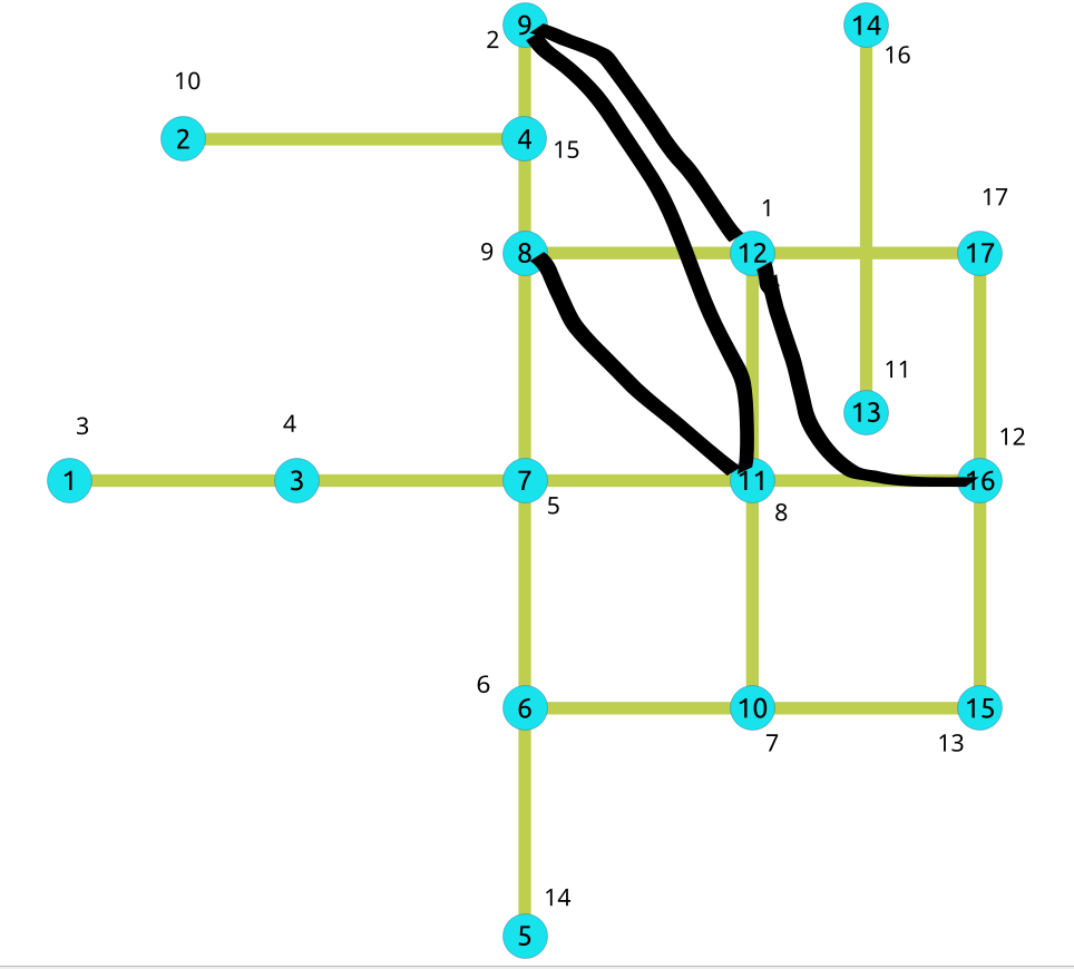
我们可以毫不意外地看到，属于捷径的顶点在结果顶点顺序中往往具有较高的优先级。

在有禁止顶点的无向图上

示例:

带有一组禁止顶点的建筑收缩

SELECT * FROM pgr_contractionHierarchies(
  'SELECT id, source, target, cost FROM edges',
  directed => false,
  forbidden => ARRAY[6]);
 type | id  | contracted_vertices | source | target | cost | metric | vertex_order
------+-----+---------------------+--------+--------+------+--------+--------------
 v    |   1 | {}                  |     -1 |     -1 |   -1 |     -1 |            4
 v    |   2 | {}                  |     -1 |     -1 |   -1 |     -1 |            8
 v    |   3 | {}                  |     -1 |     -1 |   -1 |     -1 |            5
 v    |   4 | {}                  |     -1 |     -1 |   -1 |      0 |           15
 v    |   5 | {}                  |     -1 |     -1 |   -1 |     -1 |           12
 v    |   7 | {}                  |     -1 |     -1 |   -1 |      0 |           13
 v    |   8 | {}                  |     -1 |     -1 |   -1 |     -1 |            7
 v    |   9 | {}                  |     -1 |     -1 |   -1 |     -3 |            1
 v    |  10 | {}                  |     -1 |     -1 |   -1 |     -1 |            6
 v    |  11 | {}                  |     -1 |     -1 |   -1 |      0 |           14
 v    |  12 | {}                  |     -1 |     -1 |   -1 |     -2 |            2
 v    |  13 | {}                  |     -1 |     -1 |   -1 |     -1 |            9
 v    |  14 | {}                  |     -1 |     -1 |   -1 |      0 |           16
 v    |  15 | {}                  |     -1 |     -1 |   -1 |     -1 |           11
 v    |  16 | {}                  |     -1 |     -1 |   -1 |     -2 |            3
 v    |  17 | {}                  |     -1 |     -1 |   -1 |     -1 |           10
 e    |  -1 | {7}                 |      6 |     11 |    2 |     -1 |           -1
 e    |  -2 | {7}                 |      6 |      8 |    2 |     -1 |           -1
 e    |  -3 | {7}                 |     11 |      8 |    2 |     -1 |           -1
 e    |  -4 | {7,8}               |      6 |      9 |    3 |     -1 |           -1
 e    |  -5 | {7,8}               |     11 |      9 |    3 |     -1 |           -1
 e    |  -6 | {8}                 |     12 |      9 |    2 |     -1 |           -1
 e    |  -7 | {7,11}              |      6 |     12 |    3 |     -1 |           -1
 e    |  -8 | {7,11}              |      6 |     16 |    3 |     -1 |           -1
 e    |  -9 | {11}                |     12 |     16 |    2 |     -1 |           -1
 e    | -10 | {7,11,12}           |      6 |     17 |    4 |     -1 |           -1
(26 rows)

收缩过程步骤详情

快捷构建过程

顶点 v 通过添加快捷边来进行收缩，替换形式为 (u, v, w) 的原路径为一条边 (u, w) 。仅当 (u, v, w) 是 u 和 w 之间唯一的最短路径时，才需要快捷边 (u, w) 。

当为给定顶点 v 添加完所有快捷边后， v 的相关边会被移除，接着对剩余图中的另一个顶点进行收缩。

这个过程对图形是破坏性的，我们会制作一个副本，以便再次对其进行整体操作。收缩过程会将所有发现的捷径添加到边集 E 中，并为每个收缩顶点赋予一个度量值。这个度量值就是所谓的 收缩层次 。

用初始顶点顺序初始化队列

对于图中的每个顶点 v ，都会建立一个 v 的收缩：

节点	相邻节点
$v$	$\{p,r,u\}$
$p$	$\{u,v\}$
$u$	$\{p,v,w\}$
$r$	$\{v,w\}$
$w$	$\{r,u\}$

相邻边被移除。

只有当通过 v 的路径是 v 的前驱和后继之间唯一的最短路径时，才会从 v 的前驱到后继构建快捷边。这里的 边差 度量值为-2。

然后收缩下面的顶点。这个过程一直持续到图中的每个节点都被收缩为止。最后，图中就不再有边了，这个过程也就结束了。

第一次收缩将给出一个顶点顺序，根据度量（边差值）按升序排列。这样就得到了一个总的顶点顺序。如果 u < v ，那么 u 就比 v 重要。算法会按此顺序将顶点保存到队列中。

现在，我们将按照这个顺序再次收缩顶点，从而构建一个层次结构。

构建最终顶点顺序

一旦建立了第一顺序，算法就会利用它再次浏览图形。对于队列中的每个顶点，算法都会模拟收缩并计算其边差。如果计算出的值大于下一个要收缩的顶点的值，算法就会把它放回队列（启发式方法）。否则，该顶点将永久收缩。

向初始图形添加快捷边

最后，算法会使用初始图形（删除边之前）并添加快捷边。这样就得到了收缩后的图形，可以使用专门的 Dijkstra 算法，该算法会考虑层次结构中节点的顺序。

使用缩略语

构建收缩

SELECT * INTO contraction_results
FROM pgr_contractionHierarchies(
  'SELECT id, source, target, cost FROM edges',
  directed => false);
SELECT 21

在现有表中添加快捷边和层级

在 vertices 和 edges 表中添加新列来存储结果：

ALTER TABLE edges
  ADD is_new BOOLEAN DEFAULT false,
  ADD contracted_vertices BIGINT[];
ALTER TABLE

ALTER TABLE vertices
  ADD metric INTEGER,
  ADD vertex_order INTEGER;
ALTER TABLE

更新并插入结果到两个表中。

INSERT INTO edges(source, target, cost, reverse_cost, contracted_vertices, is_new)
  SELECT source, target, cost, -1, contracted_vertices, true
  FROM contraction_results
  WHERE type = 'e';
INSERT 0 4

UPDATE vertices
  SET metric = c.metric, vertex_order = c.vertex_order
  FROM contraction_results c
  WHERE c.type = 'v' AND c.id = vertices.id;
UPDATE 17

对其使用 Dijkstra 最短路径算法

然后，你可以使用任何类似Dijkstra的算法，等待适应的算法，它将考虑构建的顶点层级。例如：

SELECT * FROM pgr_bdDijkstra(
  'SELECT id, source, target, cost, reverse_cost FROM edges',
  1, 17
);
 seq | path_seq | node | edge | cost | agg_cost
-----+----------+------+------+------+----------
   1 |        1 |    1 |    6 |    1 |        0
   2 |        2 |    3 |    7 |    1 |        1
   3 |        3 |    7 |    8 |    1 |        2
   4 |        4 |   11 |   11 |    1 |        3
   5 |        5 |   12 |   13 |    1 |        4
   6 |        6 |   17 |   -1 |    0 |        5
(6 rows)

另请参阅

• 收缩 - 函数族

索引和表格

• Index

• Search Page