Unsupported versions:2.6 2.5 2.4 2.3
pgr_TSPeuclidean
pgr_TSPeuclidean- Approximation using metric algorithm.
Availability:
Version 4.0.0
Simulated Annealing signature removed
Results change depending on input order
Version 3.2.1
Using Boost: metric TSP approx
Simulated Annealing Algorithm no longer supported
The Simulated Annealing Algorithm related parameters are ignored: max_processing_time, tries_per_temperature, max_changes_per_temperature, max_consecutive_non_changes, initial_temperature, final_temperature, cooling_factor, randomize
Version 3.0.0
Name change from pgr_eucledianTSP
Version 2.3.0
New official function.
Description
Problem Definition
The travelling salesperson problem (TSP) asks the following question:
Given a list of cities and the distances between each pair of cities, which is the shortest possible route that visits each city exactly once and returns to the origin city?
Characteristics
This problem is an NP-hard optimization problem.
Metric Algorithm is used
Implementation generates solutions that are twice as long as the optimal tour in the worst case:
Graph characteristics for best performance:
Graph is undirected
Graph is fully connected
Graph where traveling costs on edges obey the triangle inequality.
The traveling costs are symmetric:
Traveling costs from
utovare just as much as traveling fromvtou
Results change depending on input order of the Coordinates SQL
Any duplicated identifier will be ignored. The coordinates that will be kept is arbitrarily.
The coordinates are quite similar for the same identifier, for example
1, 3.5, 1
1, 3.499999999999 0.9999999
The coordinates are quite different for the same identifier, for example
2, 3.5, 1.0
2, 3.6, 1.1
 Boost Graph Inside
Signatures
Summary
[start_id, end_id])(seq, node, cost, agg_cost)- Example:
With default values
SELECT * FROM pgr_TSPeuclidean(
  $$
  SELECT id, st_X(geom) AS x, st_Y(geom)AS y  FROM vertices ORDER BY id
  $$);
 seq | node |      cost      |   agg_cost
-----+------+----------------+---------------
   1 |    1 |              0 |             0
   2 |    6 |   2.2360679775 |  2.2360679775
   3 |    5 |              1 |  3.2360679775
   4 |   10 |  1.41421356237 | 4.65028153987
   5 |    7 |  1.41421356237 | 6.06449510225
   6 |    2 |  2.12132034356 | 8.18581544581
   7 |    9 |  1.58113883008 | 9.76695427589
   8 |    4 |            0.5 | 10.2669542759
   9 |   14 |  1.58113883009 |  11.848093106
  10 |   17 |  1.11803398875 | 12.9661270947
  11 |   16 |              1 | 13.9661270947
  12 |   15 |              1 | 14.9661270947
  13 |   11 |  1.41421356237 | 16.3803406571
  14 |   13 | 0.583095189485 | 16.9634358466
  15 |   12 | 0.860232526704 | 17.8236683733
  16 |    8 |              1 | 18.8236683733
  17 |    3 |  1.41421356237 | 20.2378819357
  18 |    1 |              1 | 21.2378819357
(18 rows)
Parameters
Parameter |
Type |
Description |
|---|---|---|
|
Coordinates SQL as described below |
TSP optional parameters
Column |
Type |
Default |
Description |
|---|---|---|---|
|
ANY-INTEGER |
|
The first visiting vertex
|
|
ANY-INTEGER |
|
Last visiting vertex before returning to
|
Inner Queries
Coordinates SQL
Column |
Type |
Description |
|---|---|---|
|
|
Identifier of the starting vertex. |
|
|
X value of the coordinate. |
|
|
Y value of the coordinate. |
Result columns
Returns SET OF (seq, node, cost, agg_cost)
Column |
Type |
Description |
|---|---|---|
seq |
|
Row sequence. |
node |
|
Identifier of the node/coordinate/point. |
cost |
|
Cost to traverse from the current
|
agg_cost |
|
Aggregate cost from the
|
Additional Examples
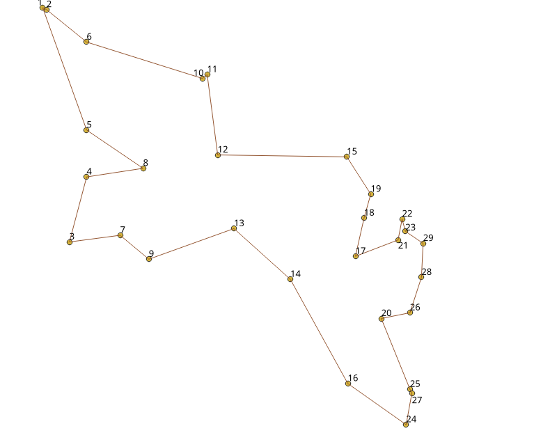
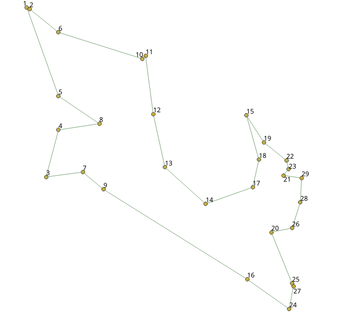
Test 29 cities of Western Sahara
This example shows how to make performance tests using University of Waterloo’s example data using the 29 cities of Western Sahara dataset
Creating a table for the data and storing the data
CREATE TABLE wi29 (id BIGINT, x FLOAT, y FLOAT, geom geometry);
INSERT INTO wi29 (id, x, y) VALUES
(1,20833.3333,17100.0000),
(2,20900.0000,17066.6667),
(3,21300.0000,13016.6667),
(4,21600.0000,14150.0000),
(5,21600.0000,14966.6667),
(6,21600.0000,16500.0000),
(7,22183.3333,13133.3333),
(8,22583.3333,14300.0000),
(9,22683.3333,12716.6667),
(10,23616.6667,15866.6667),
(11,23700.0000,15933.3333),
(12,23883.3333,14533.3333),
(13,24166.6667,13250.0000),
(14,25149.1667,12365.8333),
(15,26133.3333,14500.0000),
(16,26150.0000,10550.0000),
(17,26283.3333,12766.6667),
(18,26433.3333,13433.3333),
(19,26550.0000,13850.0000),
(20,26733.3333,11683.3333),
(21,27026.1111,13051.9444),
(22,27096.1111,13415.8333),
(23,27153.6111,13203.3333),
(24,27166.6667,9833.3333),
(25,27233.3333,10450.0000),
(26,27233.3333,11783.3333),
(27,27266.6667,10383.3333),
(28,27433.3333,12400.0000),
(29,27462.5000,12992.2222);
Adding a geometry (for visual purposes)
UPDATE wi29 SET geom = ST_makePoint(x,y);
Total tour cost
Getting a total cost of the tour, compare the value with the length of an optimal tour is 27603, given on the dataset
SELECT *
FROM pgr_TSPeuclidean($$SELECT * FROM wi29 ORDER BY id$$)
WHERE seq = 30;
 seq | node |     cost      |   agg_cost
-----+------+---------------+---------------
  30 |    1 | 2266.91173136 | 28777.4854127
(1 row)
Getting a geometry of the tour
WITH
tsp_results AS (SELECT seq, geom FROM pgr_TSPeuclidean($$SELECT * FROM wi29$$) JOIN wi29 ON (node = id))
SELECT ST_MakeLine(ARRAY(SELECT geom FROM tsp_results ORDER BY seq));
                                                                                                                                                                                                                                                                                                                                                                                                                                                                                                    st_makeline
--------------------------------------------------------------------------------------------------------------------------------------------------------------------------------------------------------------------------------------------------------------------------------------------------------------------------------------------------------------------------------------------------------------------------------------------------------------------------------------------------------------------------------------------------------------------------------------------------------------------------------------------------------------------------------------------------------------------------------------------------------------------------------------------------------------------------------------------------------------------------------------------------------------------------------------------------------------------------------------------------------------------
 01020000001E000000F085C9545558D4400000000000B3D040000000000069D440107A36ABAAAAD040000000000018D54000000000001DD040107A36AB2A10D7401FF46C5655FDCE40000000000025D740E10B93A9AA1ECF40F085C954D552D740E10B93A9AA62CC40107A36ABAA99D7400000000000E1C940107A36AB4A8FD840E10B93A9EA26C840F085C954D5AAD9401FF46C5655EFC840F085C95455D0D940E10B93A9AA3CCA40F085C9545585D940000000000052CC400000000080EDD94000000000000DCB40A52C431C0776DA40E10B93A9EA33CA40A52C431C6784DA40E10B93A9AAC9C940A52C431C8764DA402C6519E2F87DC94000000000A0D1DA4096B20C711C60C940F085C95455CADA40000000000038C840F085C9545598DA40E10B93A9AA03C740F085C954551BDA40E10B93A9AAD1C640F085C9545598DA40000000000069C440107A36ABAAA0DA40E10B93A9AA47C440107A36ABAA87DA40E10B93A9AA34C340000000008089D94000000000009BC440F085C954D526D6401FF46C5655D6C840F085C954D5A9D540E10B93A9AAA6C9400000000000CDD4401FF46C56556CC940000000000018D5400000000000A3CB40F085C954D50DD6400000000000EECB40000000000018D5401FF46C56553BCD40F085C9545558D4400000000000B3D040
(1 row)
Visual results
Visually, The first image is the optimal solution and the second image
is the solution obtained with pgr_TSPeuclidean.
See Also
Indices and tables