
Versiones no soportadas:2.6 2.5 2.4 2.3
Supported versions:
pgr_TSPeuclidean
pgr_TSPeuclidean- Aproximation using metric algorithm.

Boost Graph Inside
Availability:
Version 3.2.1
Metric Algorithm from Boost library
Simulated Annealing Algorithm no longer supported
The Simulated Annealing Algorithm related parameters are ignored: max_processing_time, tries_per_temperature, max_changes_per_temperature, max_consecutive_non_changes, initial_temperature, final_temperature, cooling_factor, randomize
Versión 3.0.0
Cambio de nombre de pgr_eucledianTSP
Versión 2.3.0
Nueva función Oficial
Descripción
Problem Definition
The travelling salesperson problem (TSP) asks the following question:
Dada una lista de ciudades y las distancias entre cada par de ciudades, que corresponde con la ruta más corta posible que para visite cada ciudad exactamente una vez y regrese a la ciudad de origen?
General Characteristics
This problem is an NP-hard optimization problem.
Metric Algorithm is used
Implementation generates solutions that are twice as long as the optimal tour in the worst case when:
Graph is undirected
Graph is fully connected
Graph where traveling costs on edges obey the triangle inequality.
On an undirected graph:
The traveling costs are symmetric:
Traveling costs from
utovare just as much as traveling fromvtou
Characteristics
Duplicated identifiers with different coordinates are not allowed
The coordinates are quite the same for the same identifier, for example
1, 3.5, 1
1, 3.499999999999 0.9999999
The coordinates are quite different for the same identifier, for example
2 , 3.5, 1.0
2 , 3.6, 1.1
Any duplicated identifier will be ignored. The coordinates that will be kept is arbitrarly.
Firmas
Resumen
pgr_TSPeuclidean(Coordinates SQL, [start_id], [end_id])
RETURNS SETOF (seq, node, cost, agg_cost)
- Ejemplo
With default values
SELECT * FROM pgr_TSPeuclidean(
    $$
    SELECT id, st_X(the_geom) AS x, st_Y(the_geom)AS y  FROM edge_table_vertices_pgr
    $$);
 seq | node |      cost      |   agg_cost
-----+------+----------------+---------------
   1 |    1 |              0 |             0
   2 |    2 |              1 |             1
   3 |    8 |  1.41421356237 | 2.41421356237
   4 |    7 |              1 | 3.41421356237
   5 |   14 |  1.58113883008 | 4.99535239246
   6 |   15 |            1.5 | 6.49535239246
   7 |   13 |            0.5 | 6.99535239246
   8 |   17 |            1.5 | 8.49535239246
   9 |   12 |  1.11803398875 | 9.61338638121
  10 |    9 |              1 | 10.6133863812
  11 |   16 | 0.583095189485 | 11.1964815707
  12 |    6 | 0.583095189485 | 11.7795767602
  13 |   11 |              1 | 12.7795767602
  14 |   10 |              1 | 13.7795767602
  15 |    5 |              1 | 14.7795767602
  16 |    4 |   2.2360679775 | 17.0156447377
  17 |    3 |              1 | 18.0156447377
  18 |    1 |  1.41421356237 |    19.4298583
(18 rows)
Parámetros
Parámetro |
Tipo |
Valores predeterminados |
Descripción |
|---|---|---|---|
Coordenadas SQL |
|
An SQL query, described in the Coordinates SQL section |
|
start_vid |
|
|
The first visiting vertex
|
end_vid |
|
|
Last visiting vertex before returning to
|
Consulta interna
Coordinates SQL
Coordenadas SQL: una consulta SQL, que debe devolver un conjunto de filas con las siguientes columnas:
Columna |
Tipo |
Descripción |
|---|---|---|
id |
|
Identifier of the starting vertex. |
x |
|
Valor X de la coordenada. |
y |
|
Valor Y de la coordenada. |
Columnas de Resultados
Devuelve el CONJUNTO DE (seq, node, cost, agg_cost)
Columna |
Tipo |
Descripción |
|---|---|---|
seq |
|
Secuencia de filas. |
node |
|
Identificador del nodo/coordenada/punto. |
cost |
|
Coste que se debe recorrer desde el
|
agg_cost |
|
Costo agregado del
|
Ejemplos Adicionales
- Ejemplo
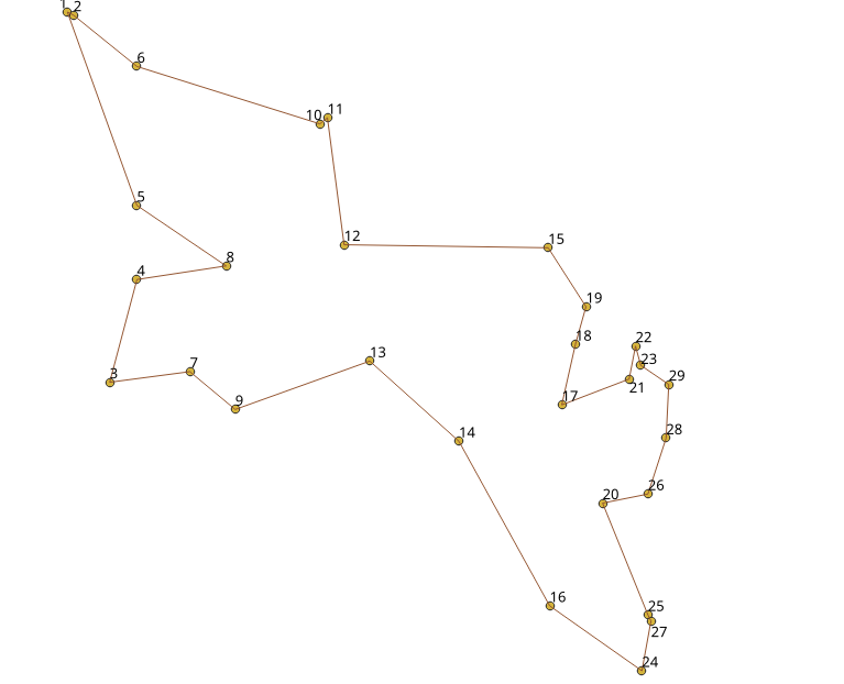
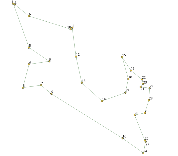
Test 29 cities of Western Sahara
This example shows how to make performance tests using University of Waterloo’s example data using the 29 cities of Western Sahara dataset
Creating a table for the data and storing the data
CREATE TABLE wi29 (id BIGINT, x FLOAT, y FLOAT, geom geometry);
INSERT INTO wi29 (id, x, y) VALUES
(1,20833.3333,17100.0000),
(2,20900.0000,17066.6667),
(3,21300.0000,13016.6667),
(4,21600.0000,14150.0000),
(5,21600.0000,14966.6667),
(6,21600.0000,16500.0000),
(7,22183.3333,13133.3333),
(8,22583.3333,14300.0000),
(9,22683.3333,12716.6667),
(10,23616.6667,15866.6667),
(11,23700.0000,15933.3333),
(12,23883.3333,14533.3333),
(13,24166.6667,13250.0000),
(14,25149.1667,12365.8333),
(15,26133.3333,14500.0000),
(16,26150.0000,10550.0000),
(17,26283.3333,12766.6667),
(18,26433.3333,13433.3333),
(19,26550.0000,13850.0000),
(20,26733.3333,11683.3333),
(21,27026.1111,13051.9444),
(22,27096.1111,13415.8333),
(23,27153.6111,13203.3333),
(24,27166.6667,9833.3333),
(25,27233.3333,10450.0000),
(26,27233.3333,11783.3333),
(27,27266.6667,10383.3333),
(28,27433.3333,12400.0000),
(29,27462.5000,12992.2222);
Adding a geometry (for visual purposes)
UPDATE wi29 SET geom = ST_makePoint(x,y);
Getting a total cost of the tour, compare the value with the length of an optimal tour is 27603, given on the dataset
SELECT *
FROM pgr_TSPeuclidean($$SELECT * FROM wi29$$)
WHERE seq = 30;
 seq | node |     cost      |   agg_cost
-----+------+---------------+---------------
  30 |    1 | 2266.91173136 | 28777.4854127
(1 row)
Getting a geometry of the tour
WITH
tsp_results AS (SELECT seq, geom FROM pgr_TSPeuclidean($$SELECT * FROM wi29$$) JOIN wi29 ON (node = id))
SELECT ST_MakeLine(ARRAY(SELECT geom FROM tsp_results ORDER BY seq));
                                                                                                                                                                                                                                                                                                                                                                                                                                                                                                    st_makeline
--------------------------------------------------------------------------------------------------------------------------------------------------------------------------------------------------------------------------------------------------------------------------------------------------------------------------------------------------------------------------------------------------------------------------------------------------------------------------------------------------------------------------------------------------------------------------------------------------------------------------------------------------------------------------------------------------------------------------------------------------------------------------------------------------------------------------------------------------------------------------------------------------------------------------------------------------------------------------------------------------------------------
 01020000001E000000F085C9545558D4400000000000B3D040000000000069D440107A36ABAAAAD040000000000018D54000000000001DD040107A36AB2A10D7401FF46C5655FDCE40000000000025D740E10B93A9AA1ECF40F085C954D552D740E10B93A9AA62CC40107A36ABAA99D7400000000000E1C940107A36AB4A8FD840E10B93A9EA26C840F085C954D5AAD9401FF46C5655EFC840F085C95455D0D940E10B93A9AA3CCA40F085C9545585D940000000000052CC400000000080EDD94000000000000DCB40A52C431C0776DA40E10B93A9EA33CA40A52C431C6784DA40E10B93A9AAC9C940A52C431C8764DA402C6519E2F87DC94000000000A0D1DA4096B20C711C60C940F085C95455CADA40000000000038C840F085C9545598DA40E10B93A9AA03C740F085C954551BDA40E10B93A9AAD1C640F085C9545598DA40000000000069C440107A36ABAAA0DA40E10B93A9AA47C440107A36ABAA87DA40E10B93A9AA34C340000000008089D94000000000009BC440F085C954D526D6401FF46C5655D6C840F085C954D5A9D540E10B93A9AAA6C9400000000000CDD4401FF46C56556CC940000000000018D5400000000000A3CB40F085C954D50DD6400000000000EECB40000000000018D5401FF46C56553BCD40F085C9545558D4400000000000B3D040
(1 row)
Visualy, The first image is the optimal solution and
the second image is the solution obtained with pgr_TSPeuclidean.
Ver también
Datos Muestra network.
Metric Algorithm from Boost library
Índices y tablas